Analysis of Sampling-Based Planners: RRTs
Continuing from my last blog post, I now want to look at the proof that the famous RRT algorithm (which stands for Rapidly-Exploring Random Tree) is probabilistically complete (and the resulting bound on sample complexity that proof yields).
On a somewhat-related note, I recently put out a preprint of my submission to IROS 2025. It examines sampling-based planning when the configuration space has discrete symmetries (such as those that arise when manipulating a symmetric object), and a key part of the paper is a theoretical analysis that suggests that various sampling-based planning algorithms should improve in performance when leveraging the underlying symmetries.
Those analyses were built upon existing bounds (like the ones in this blog post and the previous one), so perhaps that gives a bit of a hint as to why I've been thinking about this stuff!
The Rapidly-Exploring Random Tree (RRT) Algorithm
Since Steven LaValle introduced the RRT algorithm in 1998, it has become one of the most widely-used motion planning algorithms across all of robotics. The algorithm itself is relatively simple. We build up a tree in configuration space, and at each iteration, we draw a random collision-free sample (usually via rejection sampling), find its closest neighbor in the tree, and try to extend the tree a little bit towards the sample (by checking for collisions along the edge between them). This last step is called expanding a node. Below, you can see a visualization of a variant of the algorithm called RRT-Connect (where we grow two RRTs, and try to link them to each other). You can also find a nice visualization here, courtesy of my advisor.
From a first glance, it may not be clear what makes RRT so special. As it turns out, other naive strategies for building the tree will lean to a sort of "hairball", not actually expanding very far. However, the RRT sampling strategy induces a so called "Voronoi bias". A Voronoi diagram is a tessellation of a space into regions induced by a point set, where each piece is defined as the set of all points which are closest to a given point. Here's an example of a Voronoi diagram from Wikipedia:

At each iteration, whichever Voronoi region the point is drawn from will determine which node in the RRT is expanded. Thus, the probability a given node is expanded is proportional to the volume of its corresponding Voronoi region. This is precisely the Voronoi bias that RRT leverages to quickly expand to fill the configuration space (and therefore find a path from the start to the goal). I personally really like this visualization of the Voronoi bias.
Analysis of the Rapidly-Exploring Random Tree Algorithm
Analyzing the RRT algorithm is more challenging than the (radius or visibility variants of the) PRM algorithm, because for any given sample, only one connection is made. So even if a new sample may have a collision-free straight-line path to a point in the tree, it might not find it if a different point in the tree is closer.
In their paper Probabilistic Completeness of RRT for Geometric and Kinodynamic Planning with Forward Propagation, Kleinbort et. al. presented a really elegant way around this challenge. Recall that a path is ϵ-clear if we can push a ball of radius ϵ along the path and not hit an obstacle. The key idea of their proof is to construct a sequence of balls along the path, and suppose that the RRT has already reached the nth ball. Then to reach the (n+1)th ball, suppose a sample is drawn from that ball. If the nearest point is the point we have in the nth ball, then they will be connected, and all is well. If that point is not the nearest point, then it must connect to some other point that is closer. By carefully defining the radius of the balls and the degree to which they overlap, one can ensure that this edge is contained entirely within the ϵ-width "corridor" along the path that is guaranteed to be collision free. Thus, the RRT reaches the (n+1)th ball (in a collision-free manner, of course), whether or not it connected via the point in the previous ball.
The exact construction is to let 𝜈 be the minimum of ϵ and η, where η is the step size used by the RRT planner. Then cover the trajectory in m+1 balls of radius 𝜈/5, whose centers are evenly-spaced, where m=5L/𝜈. From here, a careful application of the triangle inequality can be used to show that if the nearest point to the sample in ball n+1 is not in ball n, then the new candidate edge must entirely lie within ϵ distance of the path.
This yields a natural probabilistic assessment of how long it takes for RRT to converge. One simply takes the number of balls needed to cover the path (and their corresponding radius), and examines the probability of drawing a sample from each one, in order. (This can be elegantly interpreted as a Markov chain.) The precise statement of the sample complexity result is
Where m is defined as above, and p is the probability that a uniform random sample is drawn from a ball of radius 𝜈/5. This demonstrates that for any fixed pair of points for which a path of some positive clearance exists, the probability that RRT hasn't found it exponentially converges to zero.
Warning: imprecision ahead! One key takeaway of this result is it gives some intuition as to why RRT seems to escape the curse of dimensionality in a way that other sampling-based planners like PRM do not. Even though the volume of a configuration space may grow exponentially with the dimension, this sample complexity result shows that, in some sense, RRT is able to fight that with exponential power of its own.
Comments
Post a Comment