Analysis of Sampling-Based Planners: PRMs
It's been a while since I've done one of these! Turns out it can be hard to find the time to blog when PhD life gets busy.
Today's blog post is the first in a series of several focused on the theoretical analysis of sampling-based planners. I'm currently making a push on an IROS paper that's dealing with sampling-based planning on a certain special class of manifolds, so I'm naturally thinking about the theoretical properties of these algorithms in that new domain. I also recently gave a short presentation to my lab about this subject, and figured I would convert those slides into a blog post.
The Probabilistic Roadmap (PRM) Algorithm
One of the most famous sampling-based planning algorithms is the probabilistic roadmap (PRM), introduced by now-Professor Lydia Kavraki in 1996. The algorithm itself is pretty simple. First, a bunch of collision free configurations are randomly sampled. Although we don't have an explicit representation of the obstacles in configuration space, we can use rejection sampling -- we check individual configurations for collisions, and discard those that aren't collision-free. Then, a local planner attempts to connect nearby configurations, building up a discrete graph. For collision-free motion planning, a common local planner will just look at the straight-line path in configuration space and check for collisions along that path with finite resolution. And "nearby" is often defined to be the k-nearest neighbors (for some fixed integer k) or the set of points within a prespecified radius. This completes the construction phase of the roadmap.
The PRM algorithm is a multi-query motion planning algorithm, which means that some amount of compute is done offline, and then the resulting work is reused to solve multiple planning queries. In the online phase of PRM, the user specifies a start and goal configuration, and these points are linked into the roadmap (often, using the same strategy is the construction phase). Thus, the motion planning problem has been reduced to graph search, and a path through the graph can be found with standard algorithms, like Dijkstra's algorithm or A* search.
 |
| A depiction of a probabilistic roadmap, taken from Lecture 15 of Michigan Robotics 320. |
Analysis of the Probabilistic Roadmap Algorithm
One key property of almost any sampling-based planning algorithm is probabilistic completeness: if a path exists between two points, then as the number of samples given to the planner increases, the probability a path hasn't been found approaches zero. The probabilistic completeness of PRM has been known for decades, but I want to specifically look at the paper Measure Theoretic Analysis of Probabilistic Path Planning, by Andrew Ladd and Lydia Kavraki. This paper, published in 2004, went beyond just proving probabilistic completeness, and actually proved a bound on the expected number of samples required to find a path.
This bound is based on the notion of path clearance. A path is ϵ-clear for some positive constant ϵ if, when the path passes closest to an obstacle, there's still a distance of at least ϵ between that point on the path and the obstacle. Another interpretation is that a path is ϵ-clear if we can push a ball of radius ϵ along the path and not hit an obstacle.
The idea behind the bound is that if a path is ϵ-clear, we can cover the path with a series of balls of radius ϵ/2. And then we can consider the probability that in N samples, we have drawn a sample from each ball. The edge connecting the points in each pair of adjacent balls will be collision free due to the path clearance, so if a sample has been drawn from each ball, we will have a path in the graph between the start and the goal.
Suppose we always draw a sample from one of the balls, but we don't know which one. By a standard lemma in probability (based on the "Coupon Collector's Problem"), the expected number of samples to draw before we have one in each ball is at most N -- the number of balls -- times H(N) -- the nth Harmonic number (which grows logarithmically with N). Factoring in the probability that a sample is drawn from one of the balls, and noting that if the length of the path is L, then we need 2L/ϵ balls to cover the path, the authors obtain the following upper bound on the expected number of samples:
 |
| Proposition V.1 of Ladd and Kavraki 2004. |
The notation μ(·) is used to denote the volume of a set and X is the collision-free space, so we can see that the ratio of the volume of free space to the volume of one of the individual balls used to cover the path is a key factor in this bound. In practice, we can't estimate the volume of the collision-free space, so the volume of the whole space can be used instead.
Overall, this bound shows that the expected number of samples to find a path between any two points is logarithmic in the ratio of the length of the path to the clearance of the path. This makes sense intuitively -- it's easier to find a shorter path, and it's easier to find a "wider" path. However, the ratio of the volume of the free space to the volume of one of the balls will increase rapidly as dimension increases, revealing the effects of the curse of dimensionality on PRMs.
Comments
Post a Comment