Manifold Learning Primer

Almost all of my research experience up to the present has been related to manifold learning, as are many of the papers I'm looking forward to breaking down on this blog. So this post represents a quick, self-contained primer on manifold learning, including the theory, practice, and why you would care about it in the robotics world.

An example of the manifold learning process, on the classic "Swiss Roll" dataset, using ISOMAP.

The Curse of Dimensionality

Broadly speaking, there is no precise definition for the "Curse of Dimensionality". It's a catchall term used by machine learning practitioners to refer to the variety of issues that can be caused by high dimensional data. In this section, I'll cover a variety of these issues, and discuss why the dimensionality of the problem specifically causes the problems.

One of the clearest examples of the curse of dimensionality is the intractability of many sampling-based probabilistic algorithms in high dimensional spaces. One such algorithm is the particle filter, a common technique used for object tracking and state estimation in robotics. With respect to the dimensionality of the problem, the number of samples needed to appropriately cover the state space grows exponentially. This means that particle filters can rarely be used for high dimensional problems.

In general, machine learning algorithms struggle when they aren't given very much data. This is especially problematic when the data is high dimensional: as the dimensionality grows, exponentially more data is required to adequately describe the various combinations of features that may be possible. In other words, for a dataset with a fixed number of samples, its sparsity grows exponentially with its dimension. As a result, people implementing machine learning algorithms have to face extra challenges in balancing the bias-variance tradeoff, and determining whether or not a model has overfit. A concrete example of this problem is the Hughes phenomenon, where at a certain point, adding more features to a dataset will actually reduce the performance of a classifier.

Another challenge associated with high dimensional data is the increasily unintuitive behavior of distance metrics. The first main challenge is that data tend to be concentrated farther away from zero. For exampe, uniformly sampled points inside a unit hypercube are much more likely to be close to a face of that hypercube, than they are to be close to the center. Another problem is that pairwise distances become less and less meaningful as dimensionality grows. Consider the problem of trying to identify the nearest neighbors to a data point. As the number of dimensions grows, the ratio of the distance to the nearest and farthest neighbor tends to 1, making this nearest-neighbors problem ambiguous.

Finally, a more practical challenge of high dimensional data relates to how a computer interfaces with a human. Our computer screens display 2D images, and our eyes see a 3D world, so it's generally impossible to directly visualize data in more than that many dimensions. Tricks like varying the color or size of data markers can help this problem, but aren't always clearly understandable. A robotics-specific challenge is the usage of human teleoperation. It's very challenging to manually operate a robot arm with even just a few degrees of freedom (hence why autonomous planning and control is a requirement in robotics).

Dimensionality Reduction

One general technique for handling high dimensional data is called "dimensionality reduction". Roughly speaking, dimensionality reduction is the process of taking data in a high dimensional space, and mapping it into a low dimensional space, while preserving the latent information within that data. "Latent information" is a somewhat vague term, and is more of a motivation than an explicit goal. Ultimately, the idea is that some useful attributes of the data will be preserved in the new representation, but how this is done varies greatly depending on the dimensionality reduction technique used. In the following paragraphs, I'll provide an overview of some common techniques (not including manifold learning -- this is deferred to a later section).

Principal Component Analysis (PCA) is a method for finding a linear projection which best preserves the variance of the dataset. Specifically, PCA is an orthogonal change of basis, so that the greatest amount of variance lies along the first dimension, and each successive dimension is the direction of greatest variance that is orthogonal to the previous dimensions. (This can be interpreted as a recursive process, where the direction of maximum variance is identified, the data are projected onto the perependicular space to that direction, and then the process is repeated, although PCA isn't actually computed in this way.) To use PCA for dimensionality reduction, one simply projects the data onto the first few dimensions of this new basis. Like many other methods in machine learning PCA can utilize the kernel method to handle nonlinearity. (In fact, many manifold learning algorithms are actually implemented as kernel PCA, with a carefully crafted kernel.)

PCA being used to project 2D data into a 1D space.

Multidimensional scaling (MDS) is a method for producing vector-space representations of data based on pairwise dissimilarities. There are several variants of MDS, but all of them try to produce an embedding that roughly preserves these dissimilarities.

Compared to more longstanding methods like PCA and MDS, autoencoders represent a more modern approch to dimensionality reduction. An autoencoder is a neural network that attempts to precisely reproduce the input data as the output data. However, the network is hourglass-shaped, with a hidden layer that has fewer neurons than the input. This forces the network to learn a compressed representation of the data, thus achieving dimensionality reduction. Autoencoders have also been used for applications beyond dimensionality reduction, including undistorting noisy data and detecting outliers.

Manifolds

Before introducing manifold learning, it's necessary to discuss what a manifold is. The idea of a manifold has been developed across centuries of mathematics, in order to generalize the properties of smooth curves and surfaces to any number of dimensions. A manifold is a topological space which is locally Euclidean -- colloquially, this means that if you look closely enough at any part of the manifold, it looks like an ordinary Euclidean space.

The formal definition of a locally Euclidean space is that about every point, there is some region around it which is homeomorphic to a Euclidean space. Two sets are said to be homeomorphic if there is a bijective map between them, that is continuous in both directions. Such a mapping is called a coordinate chart, and a collection of overlapping coordinate charts that collectively cover the manifold is called an atlas. This lines up well with its ordinary definition, as a collection of maps of parts of regions of the Earth, which together cover the entire planet. Where two charts in an atlas overlap, it's possible to pick a point in the image of one chart, and determine where it will appear in the image of the overlapping chart. This process yields a function on the region of overlap, called a transition map.

Two overlapping charts and their transition map.

In this blog post, we will exclusively be dealing with smooth manifolds (also called differentiable manifolds), which require that all of the transition mappings are infinitely differentiable. This additional piece of structure has the incredibly powerful outcome that virtually all tools of calculus in ordinary Euclidean spaces can now be used on manifolds, including differentiation and integration. It also allows the construction of the tangent space at each point in the manifold: a generalization of the idea of a tangent line to a curve, or tangent plane to a surface. Common examples of smooth manifolds include smooth curves and surfaces in 3D, and also more abstract examples like the set of all rotations in 3D space and the space of all invertible n-by-n matrices.

Manifold Learning

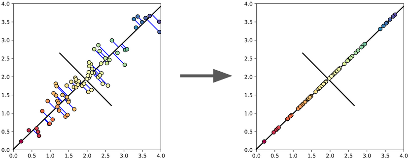
The key connection between the theory of manifolds and dimensionality reduction is the so-called manifold assumption. The manifold assumption states that high dimensional data lies along some smooth manifold of a lower intrinsic dimension. Thus, by identifying this manifold, it's possible to describe the data using the image of the manifold under a coordinate chart, requiring fewer dimensions. Colloquially, this can be thought of as unwrapping the manifold, or flattening it out, into a lower dimensional space.

To visualize this process, imagine points lying along a piece of string in 3D space. Although these points have a 3D position, they can be completely described by their position along the length of the string, which only requires one dimension. The key challenge of manifold learning is the manifold is unknown: we don't know what curve the points lie along, we simply assume one exists. So manifold learning has to discover whatever unknown manifold the data lie along, and construct a transformation of that data into a lower dimensional space based on that manifold.

The exact manner in which manifold learning attempts to unwrap the data varies depending on the algorithm. Due to the high level of structure the manifold assumption implies, there are many different properties of the manifold which can be exploited for this purpose. Here are a few of the most well-known manifold learning algorithms:

• ISOMAP connects each point to its nearest neighbors, to build up a neighborhood graph. It then estimates the geodesic distances between points (i.e. the distance along the manifold) as the shortest paths along this graph, and then uses MDS to find a low-dimensional embedding that preserves these distances.
  
• Locally-Linear Embedding (LLE) also begins by constructing a neighborhood graph, and then describes each point as a linear combination of its neighbors. By solving an eigenvalue problem, LLE then produces a low-dimensional embedding such that the weights of these linear combinations still accurately describe each point.
• Local Tangent Space Alignment (LTSA) also begins by constructing a neighborhood graph, and then estimates the tangent space at each point by performing PCA on its local neighborhood. It then produces an embedding in which these tangent spaces are aligned.
• Laplacian Eigenmaps also begins by constructing a neighborhood graph, and then computes the Laplacian of this graph. The graph Laplacian can be viewed as a discrete approxiamtion of the Laplace-Beltrami operator on a manifold; this operator has the key property that its eigenfunctions are those which best preserve locality of the data. Thus, solving the eigenvalue problem for the graph Laplacian yields a locality-preserving embedding.
  

It's also worth mentioning t-Distributed Stochastic Neighbor Embedding (t-SNE) and Uniform Manifold Approximation and Projection (UMAP). These algorithms blur the line between dimensionality reduction and data visualization, but both have mathematical motivations, and are capable of taking advantage of the manifold assumption (especially in the case of UMAP). They're also particularly good at producing nice, low-dimensional visualizations for even highly complicated datasets.

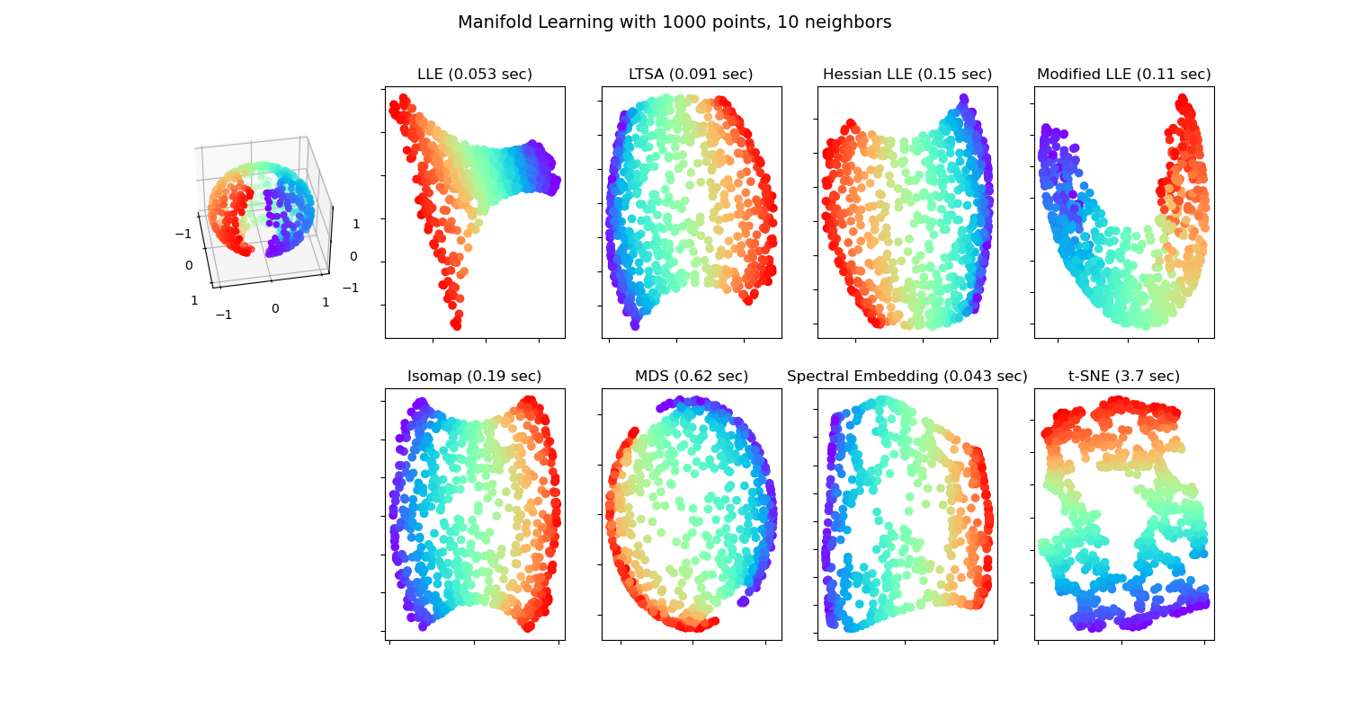The output of various manifold learning algorithms on a "severed sphere" dataset. Spectral Embedding refers to Laplacian Eigenmaps, and several modified versions of LLE are also shown.

Manifold Learning in Robotics

Oftentimes, the physical processes a robot is trying to observe or model will produce high-dimensional data that vary continuously. Thus, the manifold assumption is a reliable assumption that can be made in robotics applications, and it's unsurprising that manifold learning has been applied in a variety of different ways. In the following paragraphs, I'll be discussing several robotics papers that inspired my interest in manifold learning.

Extracting Postural Synergies for Robotic Grasping (Javier Romero et. al.) utilizes manifold learning to represent the ways that an object is grasped with a human hand. They were able to learn a latent model that describes the mechanics of the human grasp, allowing the analysis and comparison of different temporal grasp sequences.

Detecting the functional similarities between tools using a hierarchical representation of outcomes (Jivko Sinapov and Alexadner Stoytchev) utilizes manifold learning to help a robot understand the relationship between different tool shapes. Based on the types of actions that could be taken with each of the tool shapes, and the possible outcomes, the robot can learn a similarity measure across different tool geometries, and then use that information to help inform what affordances a given tool might have.

A Probabilistic Framework for Learning Kinematic Models of Articulated Objects (Jürgen Sturm et. al.) describes a general framework for the unsupervised learning of kinematic models for articulated objects. In many cases, the joint kinematics can be clearly described as rotational or prismatic. For irregular or complex joints, manifold learning was used to produce nonparametric kinematic models.

Neighborhood denoising for learning high-dimensional grasping manifolds (Aggeliki Tsoli and Odest Chadwicke Jenkins) presents a denoising technique for manifold learning, where potentially false edges

These last two papers were particularly inspiring to me; the neighborhood denoising paper directly led to TSBP: Tangent Space Belief Propagation for Manifold Learning, and the learning kinematic models paper gave me the initial idea for an experiment in Topologically-Informed Atlas Learning. I think there is definitely further potential for manifold learning's use in robotics, and I'm excited to see how it's used next. And of course, if you're reading this, I hope this guide served as a helpful introduction to moanifold learning!